Parallel Processing:

Parallel processing is a term used to denote a large class of techniques that are used to provide simultaneous data-processing tasks for the purpose of increasing the computational speed of a computer system. Instead of processing a single instruction at a time, a parallel processing system is able to process multiple instructions at a time. The purpose of parallel processing is to speed up the computer processing capability and increase its throughput (i.e. the amount of processing that can be accomplished during a given interval of time). The amount of hardware increases with parallel processing so, the cost of the system increases.

In the above figure we can see that the data stored in the processor registers is being sent to separate devices based on operation to be performed on data. If the data inside processor register is requesting for arithmetic operation, then the data will be sent to arithmetic unit. Similarly if it is requesting for logical operation, then the data will be sent to logic unit. Now, in the same time, both arithmetic operations and logical operations are executing in parallel. This is called parallel processing.

Instruction stream → The sequence of instructions read from memory is called an instruction stream.

 Data stream → The operations performed on the data in the processor is called as data stream.

 The computers are classified into 4 types based on the Instruction stream and Data stream, they are called as the Plynns Classification of computers.

Plynns Classification of Computers:
Plynns classification divides computer into four major groups as follows:

• Single instruction stream, single data stream (SISD)
• Single instruction stream, multiple data stream (SIMD)
• Multiple instruction stream, single data stream (MISD)
• Multiple instruction stream, multiple data stream (MIMD)

SISD → SISD represents the organization of a single computer, containing a control unit, a processor unit, and a memory unit. Instructions are executed sequentially and the system may or may not have internal processing capabilities. Parallel functional units or by pipeline processing.

SIMD → SIMD represents an organization that includes many processing units under the supervision of a common control unit. All processors receive the same instruction from the control unit but operate on different items of data.

MISD → MISD structure is only of theoretical interest since no practical system has been constructed using this organization.

MIMD → MIMD organization refers to a computer system capable of processing several programs at the same time. Most multiprocessor and multi-computer systems can be classified in this category.

Pipelining

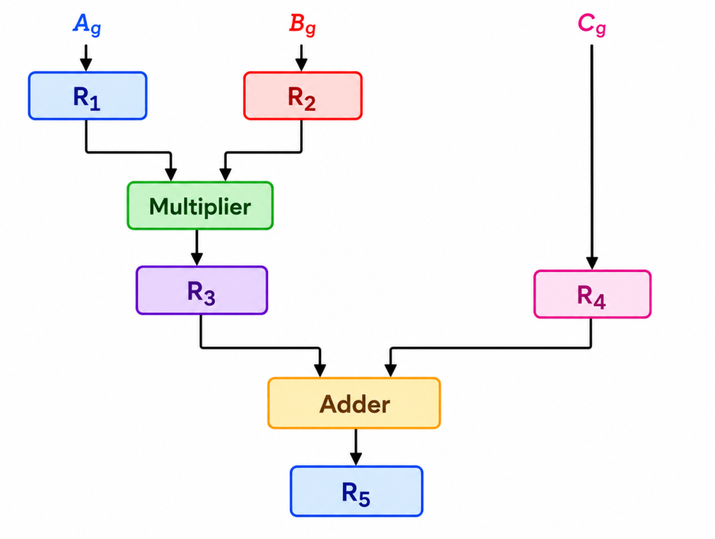
Pipelining is a technique of decomposing a sequential process into suboperations, with each subprocess being executed in a special dedicated segment that operates simultaneously with all other segments. The overlapping of computation is made possible by associating a register with each segment in the pipeline. The registers provide isolation between each segment so that each can operate on distinct data simultaneously.

Consider the operation:

Result = (A + B) × C

• First the A and B values are fetched, which is “Fetch Operation”.
• The result of the fetch operations is given as input to the addition operation, which is “Arithmetic operation”.
• The result of the arithmetic operation is again multiplied to data operand C, which is fetched from memory, which is another “Arithmetic operation”.

In this process we are using up to 5 pipelines which are:

1. Fetch operation (A)
2. Fetch operation (B)
3. Addition of (A + B)
4. Fetch operation (C)
5. Multiplication of ((A + B), C)
6. Load ((A + B) × C), Result.

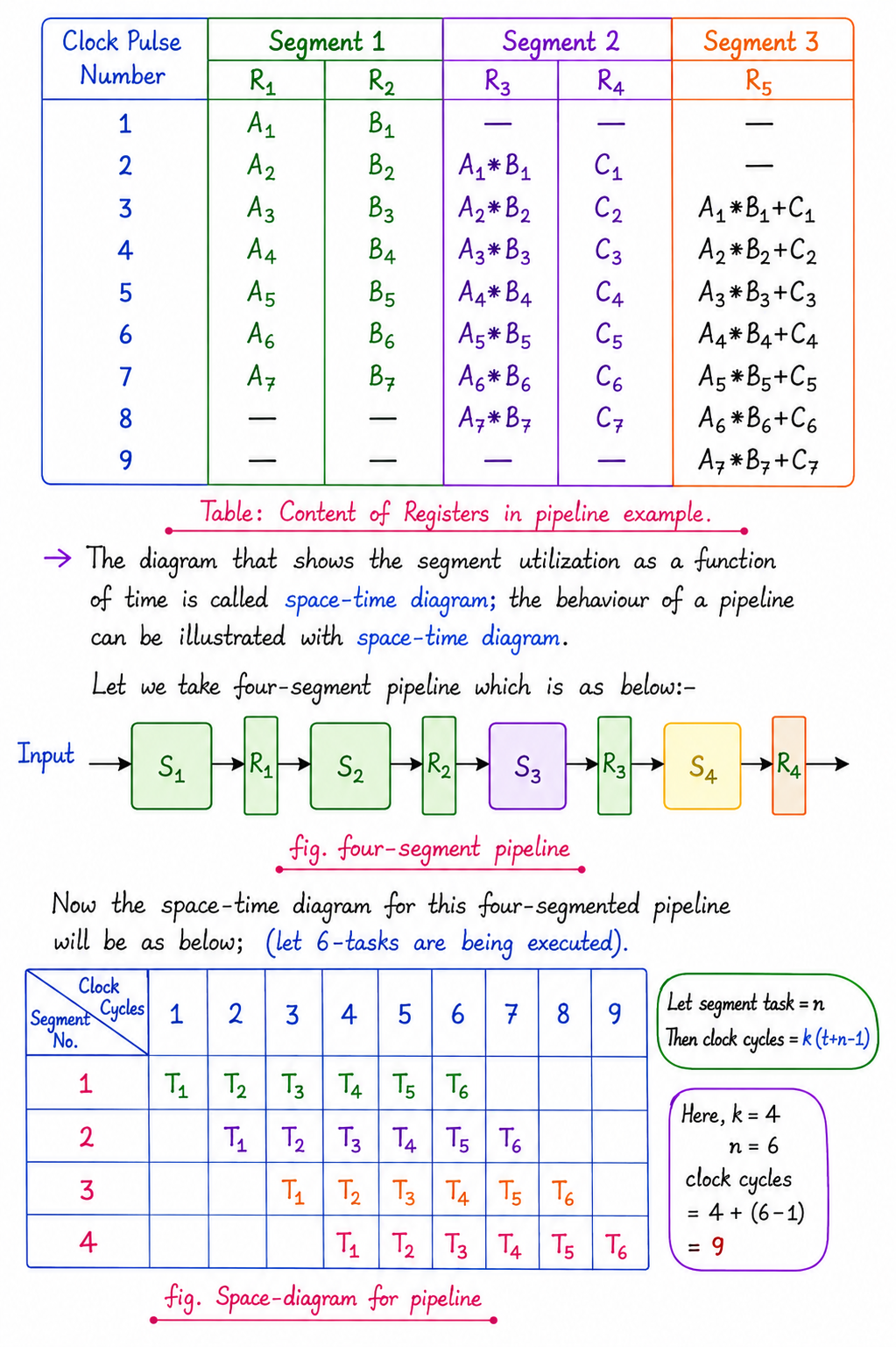
Speedup Equation

Consider there are k-segment pipelines with clock cycle time tpt_ptp​ to execute n tasks. The first task T1T_1T1​ requires a time equal to ktpk t_pktp​ to complete its operation since there are k segments. The remaining $n-1$ tasks emerge at the rate of one task per clock cycle and they will be completed after (n−1)tp​. Therefore, to complete n tasks using a k-segment pipeline requires:

k+(n−1)

clock cycles.

Example: To complete 6 tasks using a 4-segment pipeline requires:

4+(6−1)=9 clock cycles

The speedup of a pipeline processing over an equivalent non-pipeline processing is defined by the ratio:

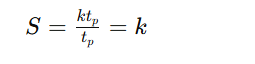
As the number of tasks increases, n becomes much larger than k − 1, and k + n − 1 approaches the value of n. Under this condition, the speedup becomes:

If we assume that the time tn taken to process a task is the same in both pipeline and non-pipeline circuits, then:

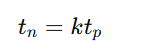
Including this assumption, the speedup reduces to:

Instruction Level Pipelining (Instruction Pipeline)

The instruction pipeline execution is like queue execution (e.g., FIFO technique). Therefore, when an instruction first arrives, it is placed in a queue and executed in the system. Finally, the result is passed to the next instruction in the queue.

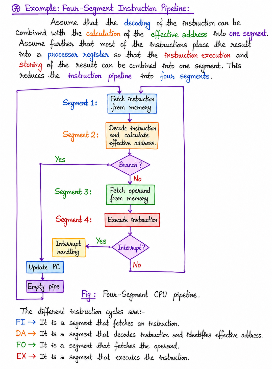
The instruction cycle is as follows:

1. Fetch the instruction from memory.
2. Decode the instruction.
3. Calculate the effective address.
4. Fetch the operands from memory.
5. Execute the instruction.
6. Store the result in the proper place.

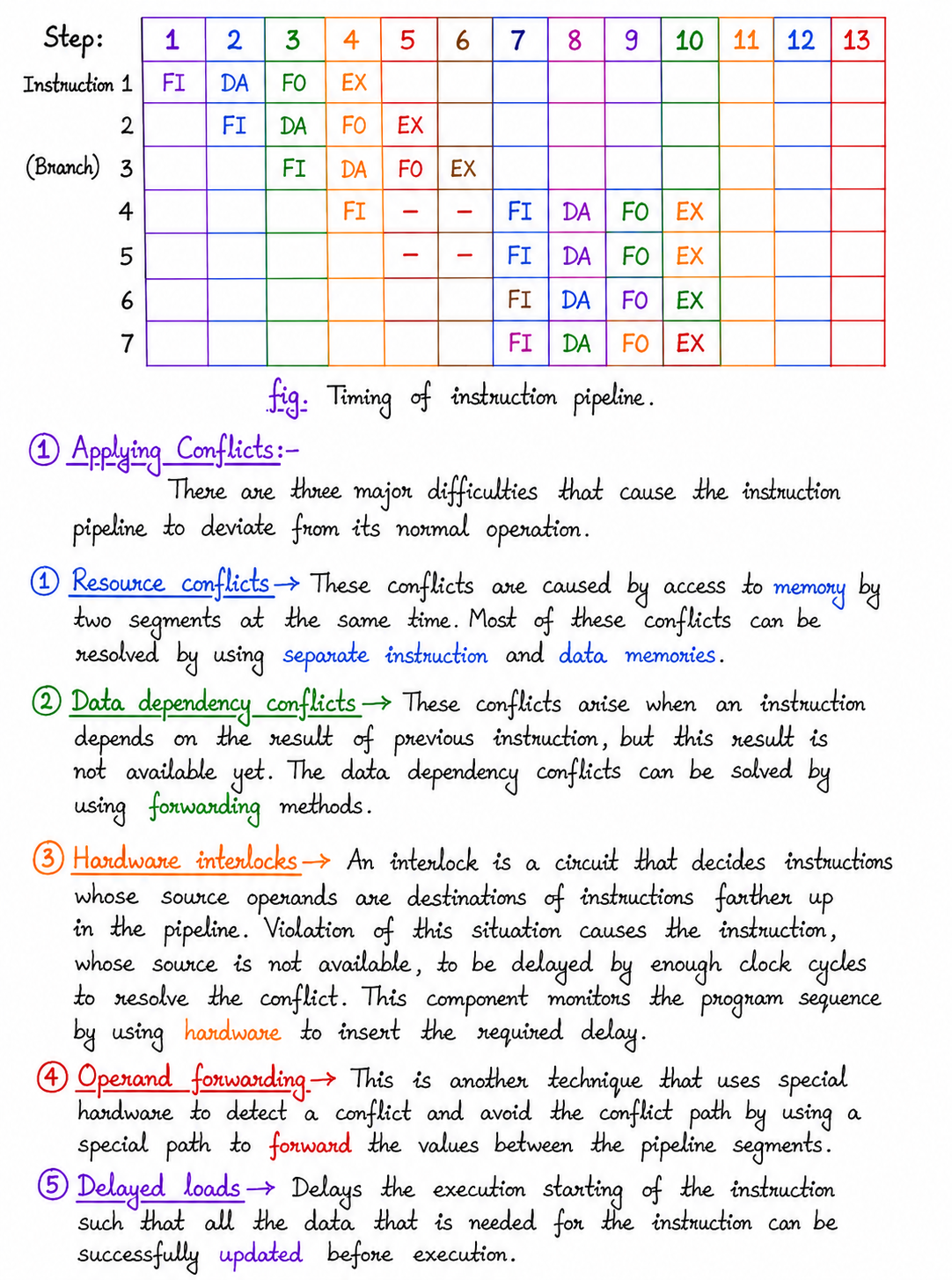
iii Branch Conflicts

These difficulties arise from branch and other instructions that change the value of the Program Counter (PC). The following are the solutions for solving branch conflicts that are obtained in the pipelining concept.

(a) Pre-fetch Target Instruction
In this method, the branch instructions that are to be executed are pre-fetched to detect if any errors are present in the branch before execution.

(b) Branch Target Buffer
It is an associative memory implemented to store branch conditions.

(c) Loop Buffer
It is a very high-speed memory device. Whenever a loop is executed in the computer, the complete loop is transferred into the loop buffer memory and is executed as in cache memory.

(d) Branch Prediction
In this method, before a branch is executed, the instructions along with the error checking conditions are checked. Therefore, unnecessary branch loops can be avoided.

(e) Delayed Branch
The delayed branch concept is similar to the delayed load process, in which the execution of a branch process is delayed before the data is fetched by the system for beginning the CPU operation.

Vector Processing

There is a class of computational problems that are beyond the capabilities of a conventional computer. These problems are characterized by the fact that they require a vast number of computations that would take a conventional computer many days or even weeks to complete. In many science and engineering applications, the problems can be formulated in terms of vectors, and this makes them suitable for vector processing.

Defⁿ: Vector processing is the process of using vectors to store a large number of variables for high-intensity data processing like weather forecasting, GIS data etc. It is a processing of sequences of data in a uniform manner with a common occurrence in manipulation of matrices or other arrays of data. The elements of those matrices are vectors.

Application areas of vector processing:

i) Long-range weather forecasting.
ii) Petroleum explorations.
iii) Seismic data analysis.
iv) Medical diagnosis.
v) Aerodynamics and space flight simulations.
vi) Artificial intelligence and expert systems.
vii) Image processing.

Vector Operations:

Many scientific problems require arithmetic operations on large arrays of numbers. These numbers are usually formulated as vectors and matrices of floating-point numbers. A vector is an ordered set of a one-dimensional array of floating-point items. A vector V of length n is represented as a row vector by
V = [V₁, V₂, V₃, …, Vₙ]

It may be represented as a column vector if the data items are listed in a column. A conventional sequential computer is capable of processing one element at a time.

Operations on vectors must be broken down into single computations with subscribed variables. The element Vi of vector V is written as V(i) and the index i refers to a memory address or register where the number is stored. Consider the following Fortran DO loop: